

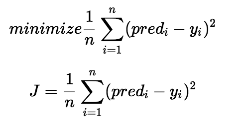
Gradient Descent is an optimization algorithm used to find the values of the parameters of any function that minimizes the cost function. The average difference of the squares of all the predicted values of y and the actual values of y is called a Cost Function. It is also called the “squared error function”, or “mean squared error”.
A cost function is a measure of how wrong the model is in terms of its ability to estimate the relationship between X and y. This is typically expressed as a difference or distance between the predicted value and the actual value of the target variable (y). The cost function can be estimated by iteratively running the model to compare estimated predictions against the known values of y.
The cost function helps us to figure out the best possible values for the coefficients (A0, A1, A2 etc.) To get the best-fit line for the data points, we would like to minimize the error between the predicted value and the actual value. The objective of a model is to find parameters that minimize the cost function.
The Ordinary Least Squares procedure seeks to minimize the sum of the squared residuals (errors). Residual (error) is the difference between the observed responses (values of the variable being predicted) in the given dataset and those predicted by a linear function of a set of explanatory variables. The smaller the differences, the better the model fits the data. Visually, this may be seen as the sum of the squared vertical distances between each data point in the set and the corresponding point on the regression line. The sum of all the squared errors together should be minima.
After estimating the values of the coefficients these values can be optimized using Gradient Descent. Gradient descent is a method of updating A0 and A1 to reduce the cost function(MSE).
We start with random values for each parameter. The goal is to continue to try different values for the parameters, evaluate their cost, and select new parameters that have a slightly lower cost. Iterating this process enough number of times leads to the values of the parameters that result in the minimum cost.
The idea is that we start with some values for A0 and A1 and then we change these values iteratively to reduce the cost. This is done by iteratively minimizing the error of the model using the training data. Gradient descent helps us how to change the values. We can measure the accuracy of the model using the cost function and so it is directly related to the performance of the model.

I have read in a technical blog that an intuitive way to think of Gradient Descent is to imagine the path of a river originating from the top of a mountain. The goal of gradient descent is exactly the same as the aim of the river, that is, to reach the foothill, the bottommost point.
Now, let us assume an ideal condition where the terrain of the mountain is such that the river does not have to stop anywhere before reaching the foothill. But, in reality, the river would face several pits on its path (these are termed as local minima solutions, which are not desirable) forcing the river to stagnate. In Machine Learning, the ideal condition of the river is similar to finding the global minimum (or optimum) of the solution.
Now, there are two important points when it comes to gradient descent; initial values and learning rate. To give a general idea about them, we know that depending on where the river initially originates, it will follow a different path to reach the foothill. Also, depending on the speed of the river (learning rate) you might arrive at the foothill in a different manner. These values are important in determining whether you will reach the foothill (global minima) or get trapped in the pits (local minima).
Gradient descent enables a model to learn the gradient or direction that the model should take in order to reduce errors (differences between actual y and predicted y). In simple linear regression, direction refers to how the model parameters should be tweaked or corrected to further reduce the cost function.
The difference between the actual and predicted values of the target data is the prediction error (E). We need to find a function with optimal values of parameters that best fit the historical data. This reduces the prediction error and improves prediction accuracy.
Sum of Squared Errors (SSE) = ½ Sum (Actual value of y – Predicted value of y)2
(the ‘1/2’ in the equation above is for mathematical convenience since it helps in calculating gradients in calculus).
The error value is calculated for each pair of input (x) and output (y) values, the error value is squared, and the sum of these squared error values is found. This value when halved gives the SSE. The process is repeated until a minimum SSE is achieved, or no further improvement is possible.
In conclusion, gradient descent is a way for us to calculate the best set of values for the parameters of concern.
The steps are as follows:
1. Given the gradient, calculate the change in parameter with respect to the size of the step taken.
2. With the new value of the parameter, calculate the new gradient.
3. Go back to step 1.
The learning rate actually refers to how large a change in the parameters we are taking. So if the gradient is steep at the standing point and you take a large step, you will see a large decrease in the cost. Alternatively, if the gradient is small (gradient is close to zero), then even if a large step is taken, given that the gradient is small, the change in the cost will be small as well.
And the sequence of steps will stop once we hit convergence. Optimization algorithms are iterative procedures. Starting from a given point, they generate a sequence of iterates that converge to a “solution”. We can say Gradient Descent is a first-order iterative optimization algorithm.
I hope this helps with your understanding of gradient descent.
Happy learning!