

There are the five major assumptions:
1. Linear relationship: There should be a linear and additive relationship between the dependent (Y) variable and the independent (X –> x1,x2,x3,…) variable(s). A linear relationship suggests that a change in response Y due to one unit change in x1 is constant, regardless of the value of x1. An additive relationship suggests that the effect of x1 on y is independent of other variables (x2,x3,…).
2. No or little multicollinearity: The independent variables (x1,x2,x3,…) should not be correlated. The presence of correlation in independent variables leads to Multicollinearity. If variables are correlated, it becomes extremely difficult for the model to determine the true effect of independent variables on the response variable, Y.
Multicollinearity can be detected using the Variance Inflation Factor (VIF). VIF of any independent variable (x1) is the ratio of the variance of its estimated coefficient in the full model to the variance of its estimated coefficient when it was fit alone.
Usually, a VIF value of above 5 or 10 is taken as an indicator of multicollinearity. A VIF of 1 indicates no presence of multicollinearity. The simplest way of getting rid of multicollinearity is to discard the independent variable with a high value of VIF.
3. No auto-correlation: There should be no correlation between the residual terms. A residual is the vertical distance between a data point and the regression line. Each data point has one residual. Residual of one observation should not predict the next observation. The Presence of correlation in error terms is known as Autocorrelation.
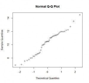
4. Normal distribution of error terms:
The fourth assumption is that the residuals follow a normal distribution. The normal distribution of the residuals can be validated by plotting a Q-Q plot. A Q-Q plot is a scatterplot created by plotting two sets of quantiles against one another. If both sets of quantiles came from the same distribution, we should see the points forming a line that’s roughly straight.
5. Homoscedasticity: It means that the residuals, the difference between the observed value and the predicted value, are equal across all values of the predictor variable.
Data is homoscedastic if the residuals plot is the same width for all values of the predicted value. Heteroscedasticity is usually shown by a cluster of points that is wider (cone shape) as the values as the predicted value get larger. In this case, some kind of variable transformation may be needed to improve model quality.


We can also use math to check homoscedasticity by checking the variance or running an F-test but the easiest way to check is to run a scatter plot and look at the data.
These assumptions are just a formal check to ensure that the linear model we build gives us the best possible results for a given data set.